
Methodology and design principles A Clarasight white paper
Forecasting Business Travel Spend and Emissions
A forecasting methodology for Finance teams to update travel spend and emissions forecasts as revenue plans, actual spend, policies, and costs change.
What's inside
- A monthly model that learns repeating patterns from historical data and refreshes as new actuals arrive.
- The spend-to-revenue ratio used to fold in revenue projections without adding model complexity.
- Three scenario types for comparing several futures side by side in one sitting.
1. Overview
Forecasting corporate travel spend and emissions is a deceptively complex problem. Travel data is seasonal, noisy, and sensitive to both business conditions and one-off events. A useful forecast has to stay stable and interpretable over a multi-year horizon, update gracefully as new actuals come in, and support scenario planning around policy levers and macroeconomic assumptions.
This paper outlines the core methodology Clarasight uses to build long-range forecasts of business travel spend and emissions. The approach is built around a deliberate set of modeling choices, each made to address a specific challenge in travel data. The result is a forecasting system that is accurate, transparent, and flexible enough to support both annual planning and mid-year monitoring.
Much of today's forecasting conversation centers on AI. Clarasight's approach draws from a broader statistical toolkit. The method in this paper is deliberately conventional: a proven statistical workhorse with visible assumptions and behavior that can be tested against actuals. For long-range planning, that predictability is a strength.
2. Why (S)ARIMA?
The foundation of the approach is the (S)ARIMA — (Seasonal) AutoRegressive Integrated Moving Average — model family. These models allow for a forecast that accounts for observed annual seasonality while keeping scenario modeling responsive enough to provide clear visibility for decision-making.
Corporate travel spend is seasonal in a way that is very company-specific. A consulting organization might see relatively consistent spend outside the holidays, while a company with conference-dependent travel sees high spend at certain times of year and little to none in others. Even within one company, billable and non-billable travel can move differently, as can spend across modalities like air and hotel. SARIMA models handle seasonality natively through their seasonal components, learning these repeating patterns from historical data rather than requiring manual adjustment. Because the model is computationally simple, generating multiple forecasts across different slices of the business — each with its own temporal pattern — is a trivial exercise.
At the same time, a long-range forecast needs to fold in year-to-date actuals to update its rest-of-year projection and pick up any shift in seasonality. SARIMA is designed for exactly this: it trains on a monthly time series and produces a monthly forecast, so a mid-year refresh simply means re-running the model on a training set that includes the recent actuals. The model structure — defined by up to six parameters — can even evolve as more data arrives: seasonal patterns get reinforced or dampened, and policy shifts soak in.
Figures 1 and 2 show what that refresh looks like when the latest five months of actual spend run 20% above the prior series: the monthly model is re-fitted on the elevated data, and the annual view shows how that change carries into projected totals.
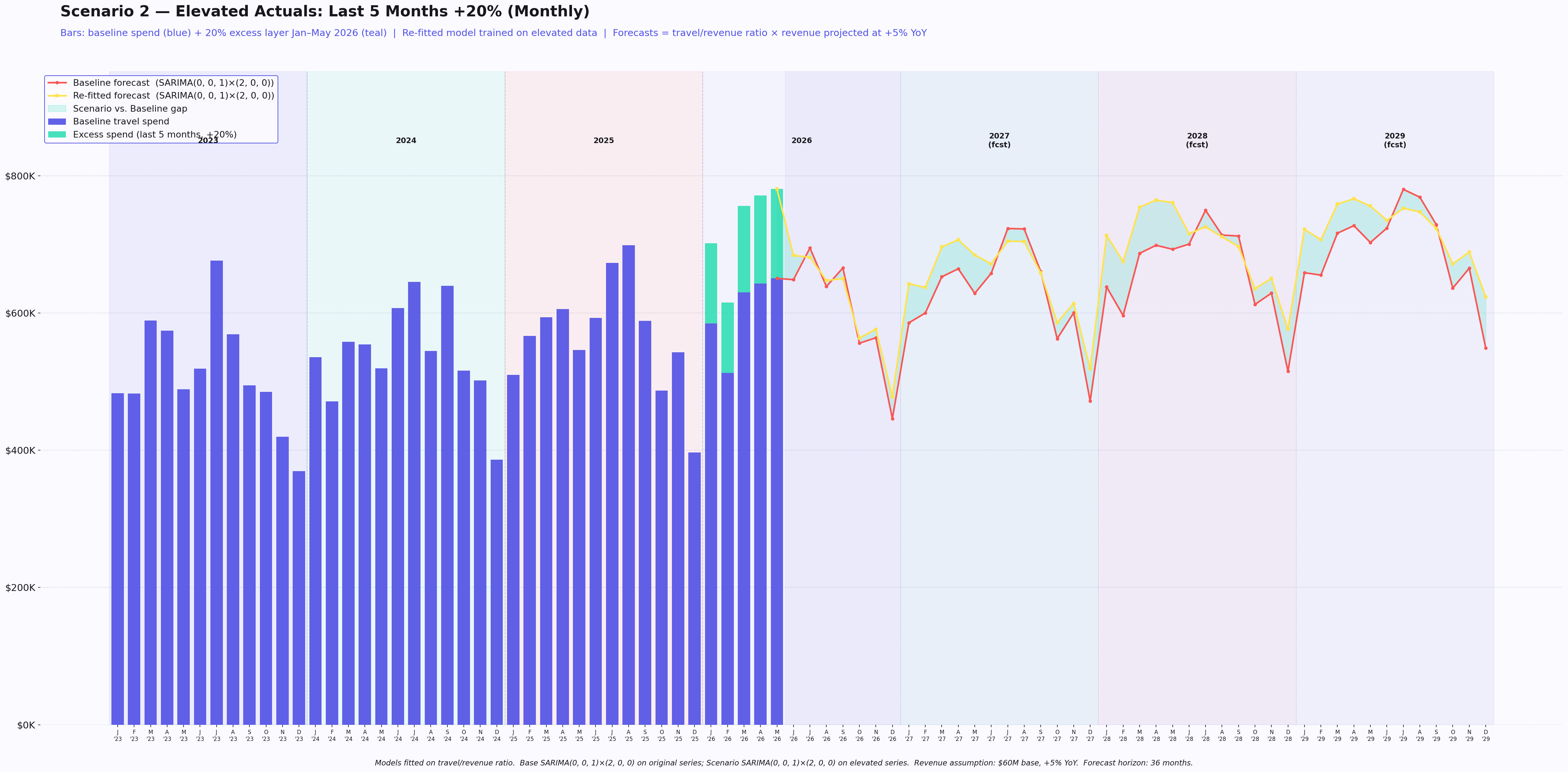
The monthly view shows a year-to-date refresh in which the latest five months of actual spend are 20% above the baseline series and the model is re-fitted on the elevated data. The data is illustrative.
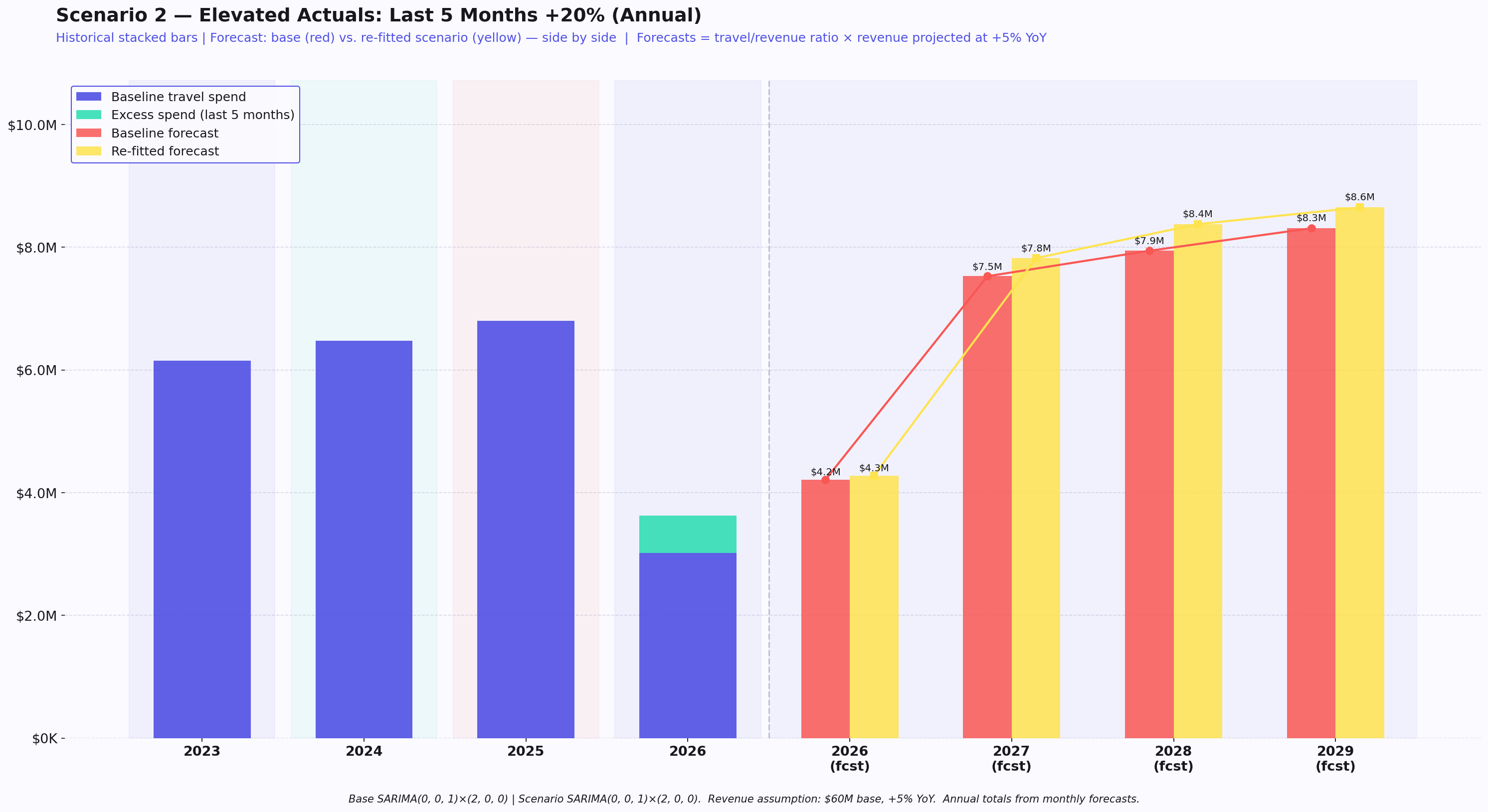
The annual view shows how the elevated year-to-date actuals carry into projected annual spend, comparing the baseline and re-fitted forecasts. The data is illustrative.
3. Prediction variables: business inputs and market forces
Prediction variables beyond time itself fall into two classes: business inputs internal to the company (endogenous variables) and market forces external to it (exogenous variables). Clarasight's forecasting tools handle the two differently.
Business inputs
Businesses often have robust internal projections for endogenous variables like headcount and revenue, driven by market research and product roadmaps. Clarasight can incorporate these directly and take a company's own projections at their word.
At Clarasight, we made the design choice to forecast the ratio of monthly spend to annual revenue (or a similar scaling variable), rather than raw spend figures directly. This decision solves several problems at once.
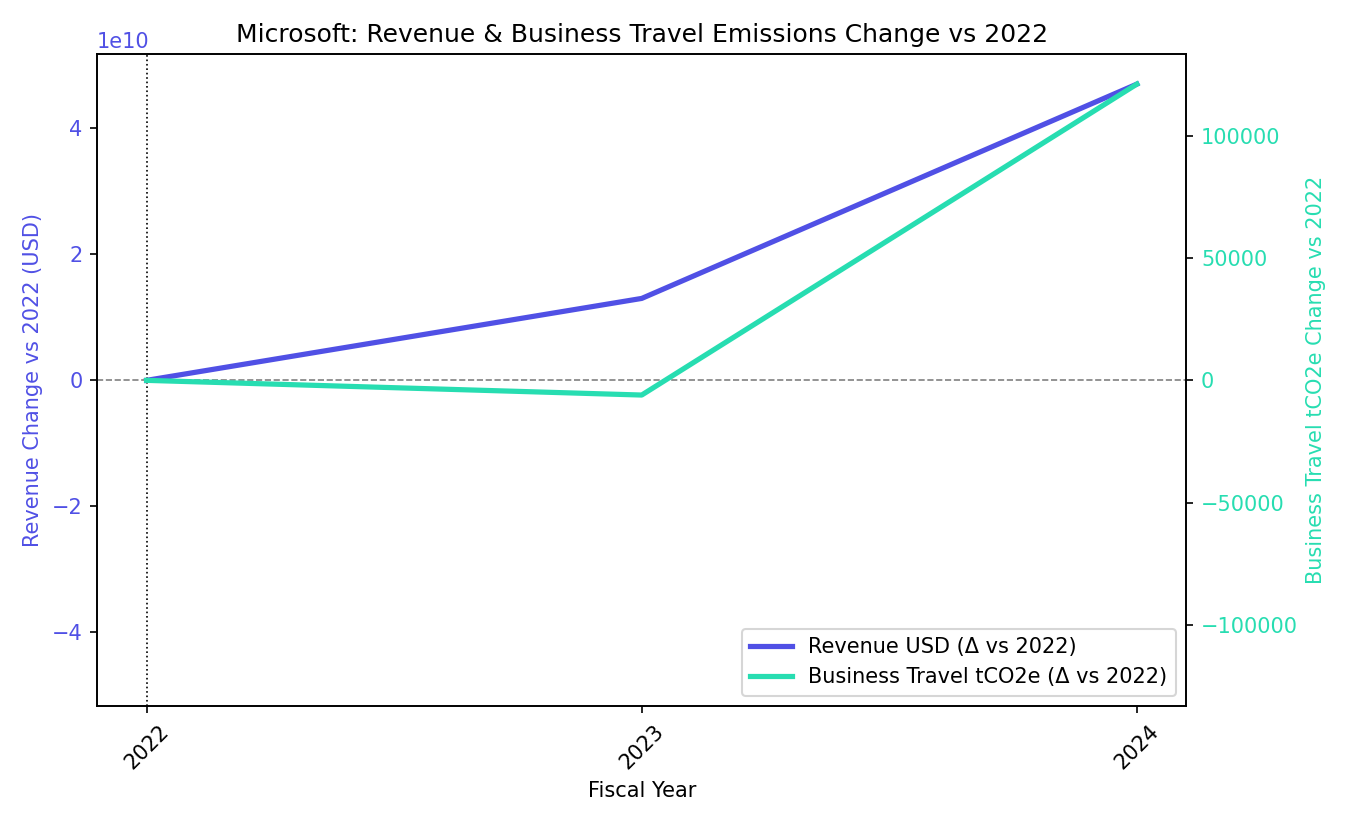
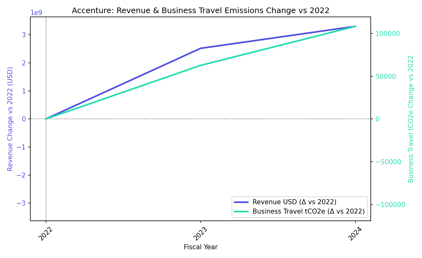
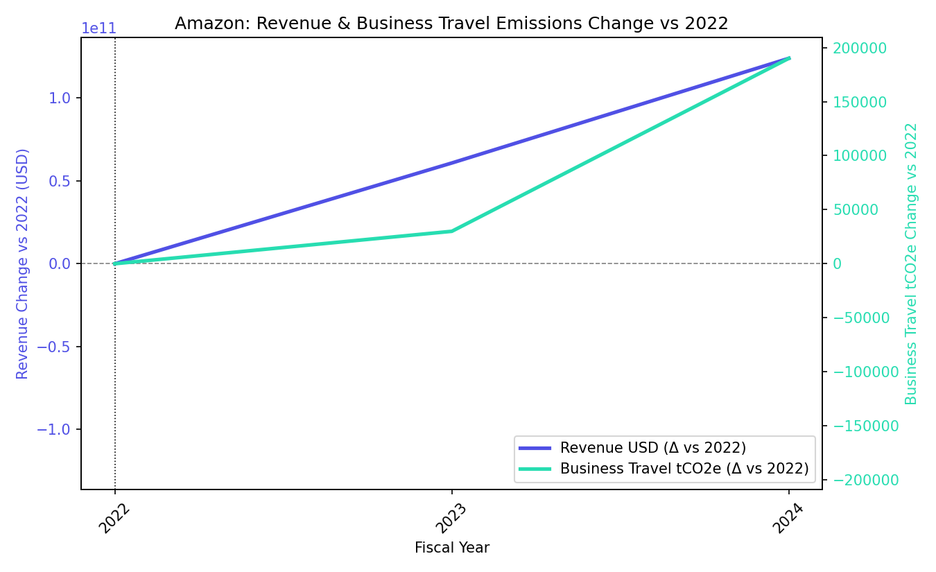
First, we have observed across several companies that raw travel spend tends to grow over time as a company grows its revenue. Comparable public data on corporate travel cost is scarce. Figure 3 therefore uses disclosed business-travel emissions as a more consistently available proxy for travel activity, paired with reported revenue. Each series shows the change from its 2022 value.
Microsoft
Accenture
Amazon
Meta
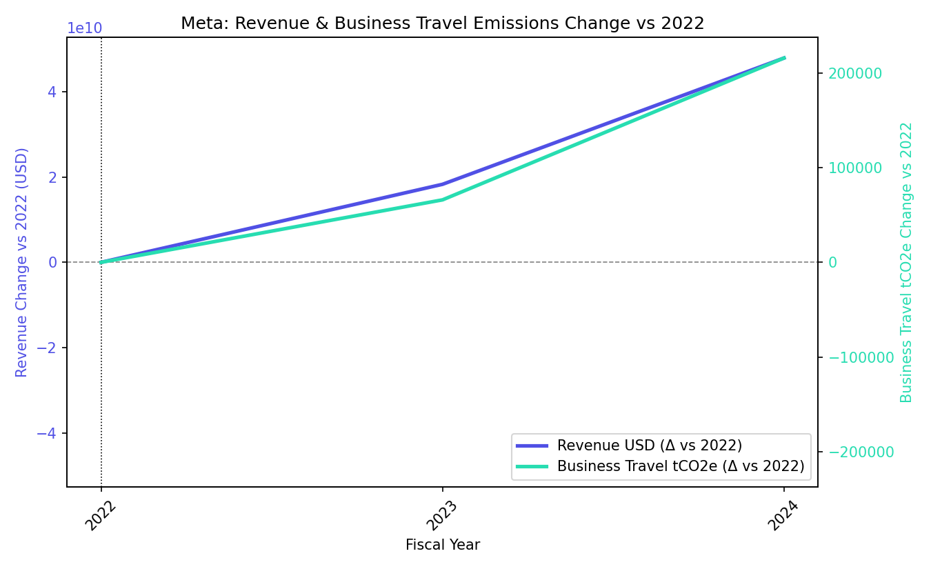
Across four panels covering Microsoft, Accenture, Amazon, and Meta, the figure plots reported revenue and disclosed business-travel emissions as the change from each company's 2022 value, drawn from public company reports. Business-travel emissions serve as a more consistently available proxy for travel activity because comparable public travel-cost data is scarce.
4. Sensitivity analysis: planning for uncertainty
Because the SARIMA framework is inexpensive to re-run, it is well suited to structured sensitivity analysis. Clarasight's forecasting supports three kinds.
Revenue sensitivity shows the impact of varying the revenue growth assumptions across a range of scenarios. Because the cost-to-revenue ratio remains identical across all growth scenarios, only the scale of the projections changes — easy to communicate a range of outcomes to business stakeholders without separate model re-runs.
Policy-change sensitivity models the impact of a structural initiative, such as shifting a class of air bookings to a lower fare category. It works by adjusting the historical training series — modifying observed data points and re-fitting the model — to quantify a counterfactual in which the policy had always been in effect. The result is a structurally similar forecast with a potentially different seasonality and cost-to-revenue ratio, useful for estimating a policy's impact in future years.
Figures 4 and 5 show that counterfactual in practice: an initiative removes roughly 10% of modeled travel spend, and the re-fitted model carries the effect from the monthly pattern into annual totals.
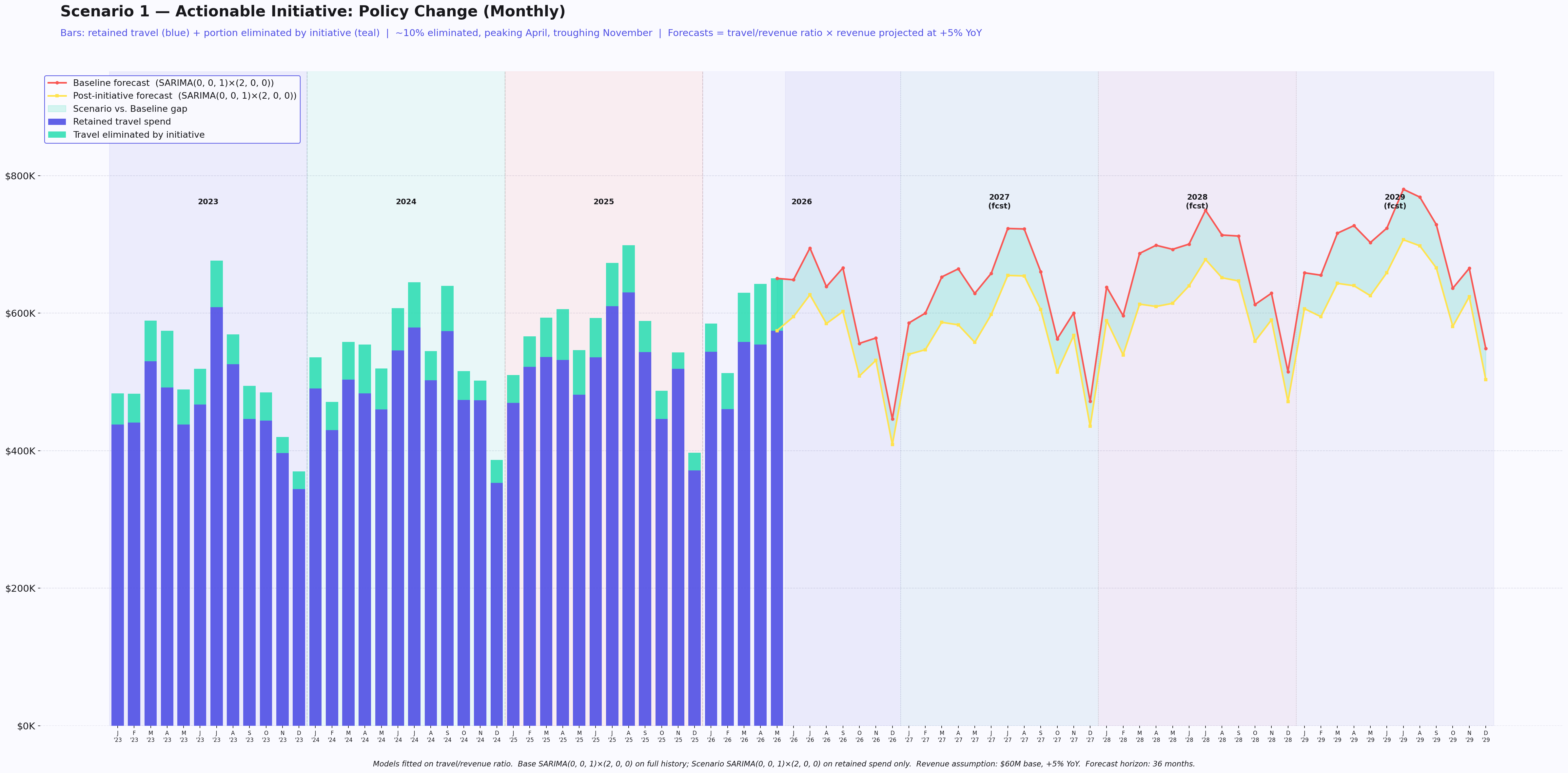
The monthly view models a policy initiative that removes roughly 10% of modeled travel spend, splitting travel into retained and eliminated portions and comparing the baseline and post-initiative forecasts. The data is illustrative.
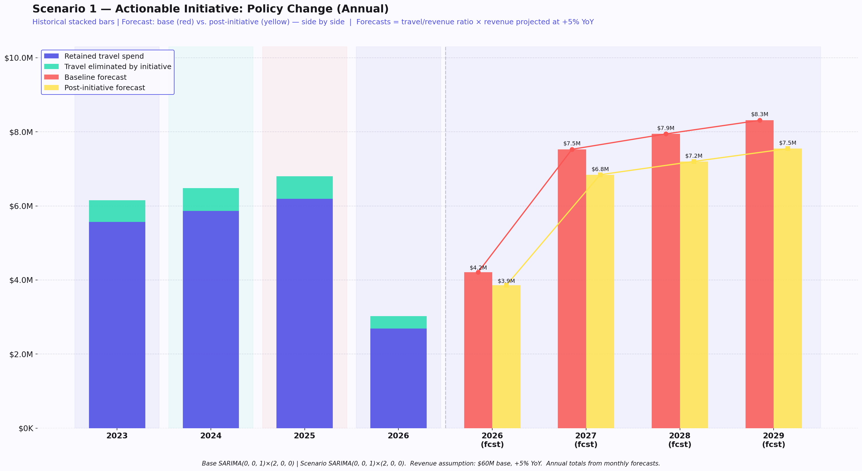
The annual view rolls the policy initiative up to yearly totals, showing historical retained and eliminated travel alongside the baseline and post-initiative annual forecasts. The data is illustrative.
Cost-shock sensitivity introduces an artificial change in one or more past or future data points, simulating a one-time event — a freeze, a policy shift, an operational shock — that drives spend anomalously low in a single month. As with a policy change, a counterfactual model is fit and used to project the shock's effect forward.
The same counterfactual method can also combine events rather than test them one at a time. Figures 6 and 7 follow a five-month 20% spend spike followed by an enforced 15% reduction through year-end, then compare the original baseline, the post-spike path, and the post-cap re-fit month by month and annually.
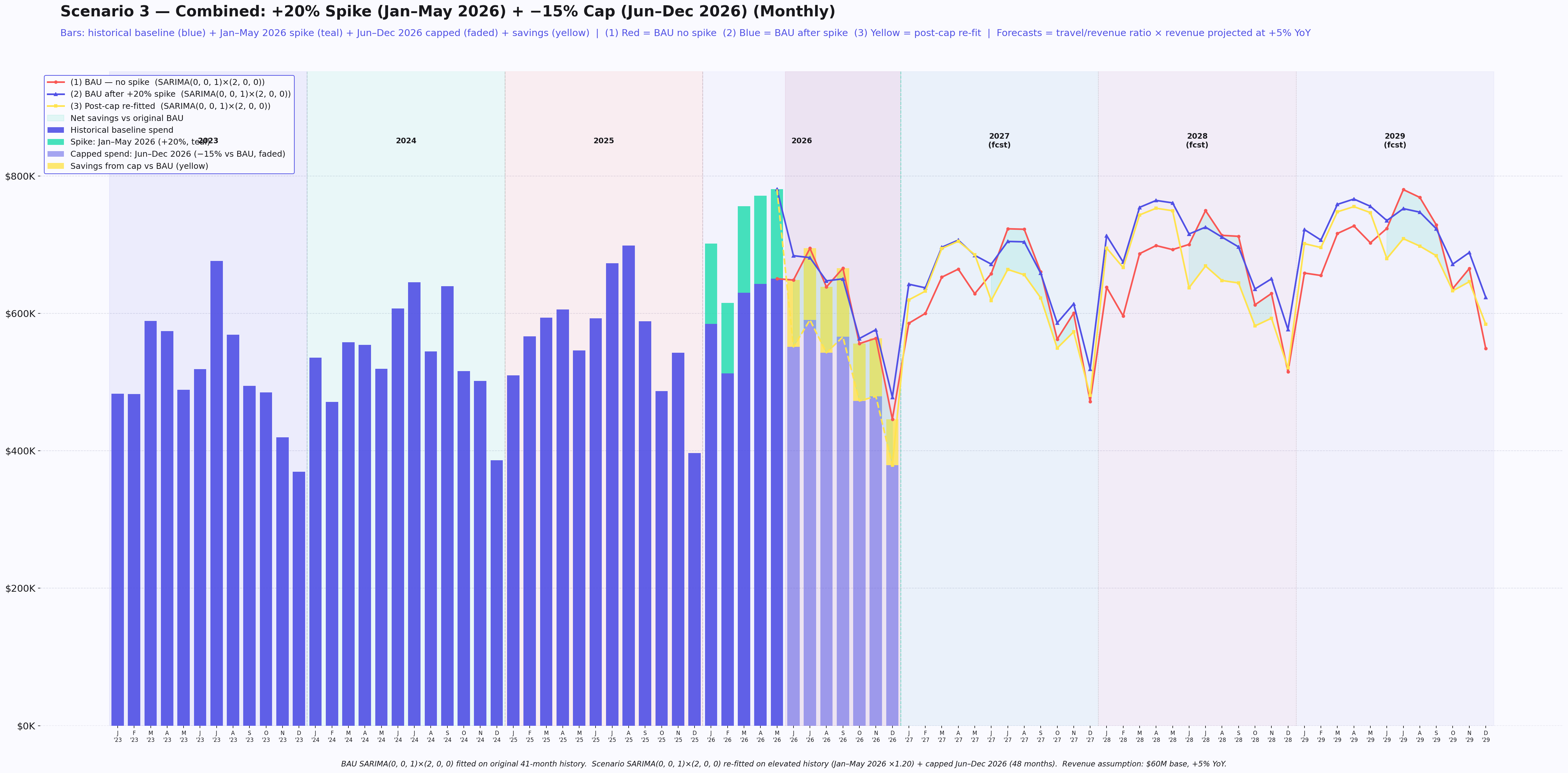
The monthly view combines two events — a 20% spend spike from January through May 2026 followed by a 15% cap from June through December — and compares the business-as-usual, post-spike, and post-cap re-fitted forecasts. The data is illustrative.
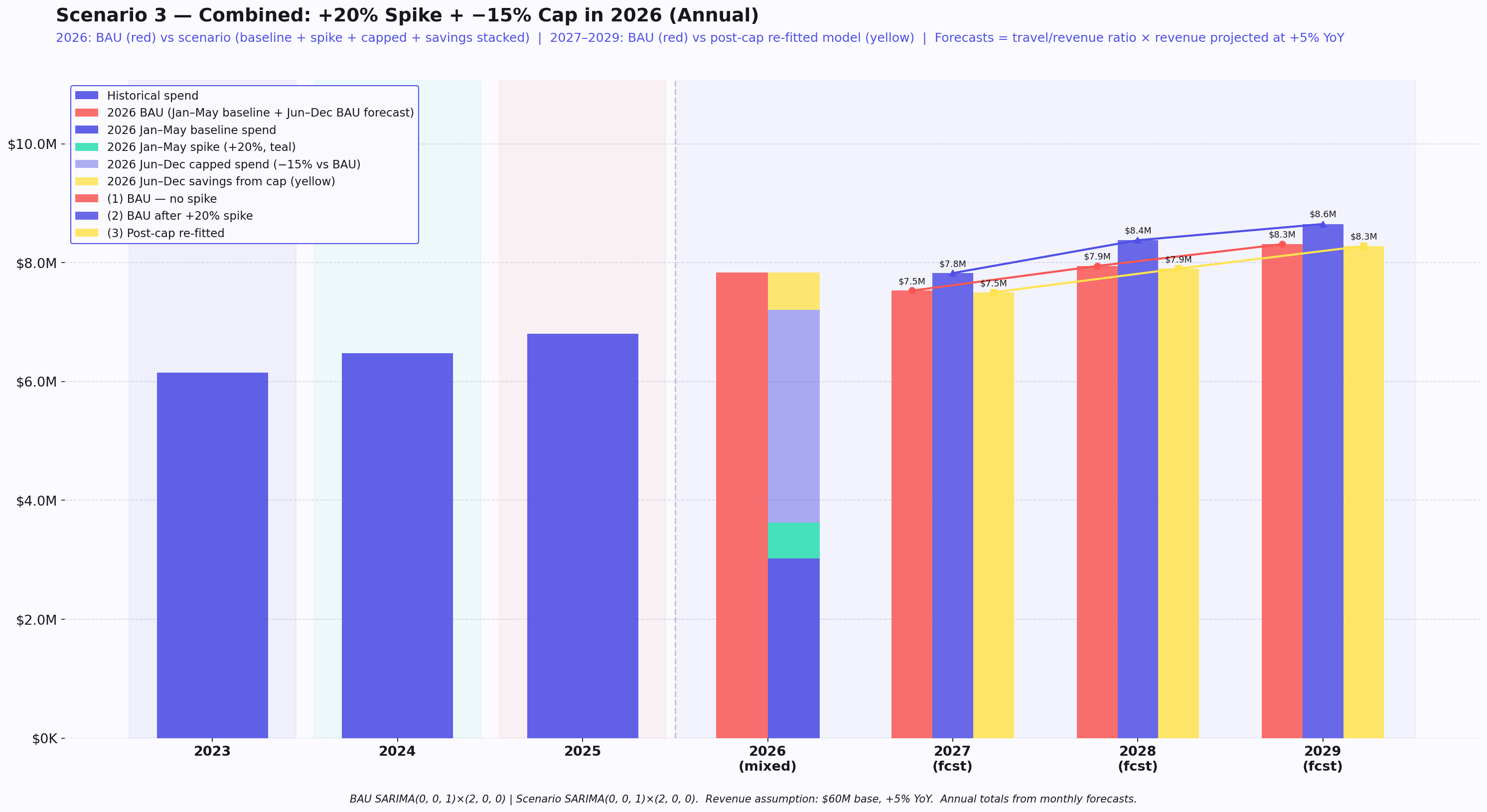
The annual view rolls the mixed 2026 spike-and-cap scenario up to annual totals across the three forecast paths. The data is illustrative.